
scipy.stats.norm is the normal distribution, and every method takes the same two arguments:
from scipy.stats import norm

norm.pdf(x, loc=0, scale=1)    # height of the curve
norm.cdf(x, loc=0, scale=1)    # probability below x
norm.ppf(p, loc=0, scale=1)    # the value with p below it
norm.rvs(size=n, loc=0, scale=1)   # random samples
loc is the mean and scale is the standard deviation. Passing a variance there is the single most common mistake, and it fails silently.
All numbers below are real output from Python 3.12.5, SciPy 1.18.1, NumPy 2.5.3.
scipy.stats.norm pdf, cdf and ppf
Three methods answer three different questions about the same curve:
from scipy.stats import norm

# the standard normal: mean 0, standard deviation 1
print("pdf(0)    :", norm.pdf(0))
print("cdf(0)    :", norm.cdf(0), "  half the area is below the mean")
print("ppf(0.5)  :", norm.ppf(0.5), "  the value with 50% below it")

print()
# loc is the MEAN, scale is the STANDARD DEVIATION
print("IQ below 110, mean 100, sd 15:", round(norm.cdf(110, loc=100, scale=15), 4))
Output:
pdf(0)    : 0.3989422804014327
cdf(0)    : 0.5   half the area is below the mean
ppf(0.5)  : 0.0   the value with 50% below it

IQ below 110, mean 100, sd 15: 0.7475| Method | Answers | Input |
|---|---|---|
pdf(x) | How tall is the curve here? | A value |
cdf(x) | What fraction is below x? | A value |
ppf(p) | Which value has p below it? | A probability |
sf(x) | What fraction is above x? | A value |
rvs(size=n) | Give me n random draws | A count |
cdf and ppf are inverses of each other, so feed one into the other and you’re back where you started.
The pdf is not a probability. Its value at a point can exceed 1 for a narrow distribution, because it is a density.
What are loc and scale in scipy.stats.norm?
scale takes the standard deviation. Give it the variance and you get a plausible, wrong answer:
from scipy.stats import norm

# scale is the standard deviation, NOT the variance
correct = norm.cdf(110, loc=100, scale=15)      # sd = 15
wrong = norm.cdf(110, loc=100, scale=225)       # 225 is the VARIANCE

print("scale=15  (std dev) :", round(correct, 6))
print("scale=225 (variance):", round(wrong, 6), "  <- wrong answer, no error")

print()
print("if you only have the variance, take its square root first:")
variance = 225
print("  scale =", variance ** 0.5)

print()
print("mean and variance back out of the distribution:")
print("  mean:", norm.mean(loc=100, scale=15), " var:", norm.var(loc=100, scale=15))
Output:
scale=15  (std dev) : 0.747507
scale=225 (variance): 0.517725   <- wrong answer, no error

if you only have the variance, take its square root first:
  scale = 15.0

mean and variance back out of the distribution:
  mean: 100.0  var: 225.0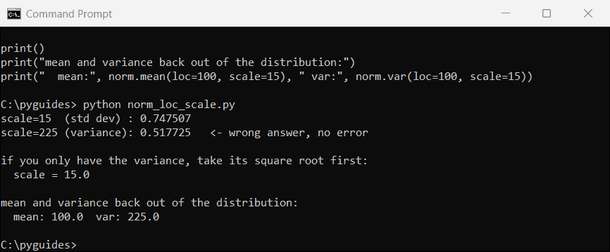
There’s no error, because 225 is a perfectly valid standard deviation. SciPy has no way to know you meant a variance.
If your data gives you a variance, take the square root before you pass it. norm.var() goes the other way when you need it back.
Plotting the normal distribution
The two curves make the relationship between pdf and cdf obvious:
import numpy as np
import matplotlib.pyplot as plt
from scipy.stats import norm

x = np.linspace(-4, 4, 400)

fig, (ax1, ax2) = plt.subplots(1, 2, figsize=(11, 4.2))

ax1.plot(x, norm.pdf(x), color="#0b6bcb", lw=2)
ax1.fill_between(x, norm.pdf(x), where=(x <= 1), alpha=.25, color="#0b6bcb")
ax1.set_title("pdf: the bell curve\nshaded area = cdf(1)")

ax2.plot(x, norm.cdf(x), color="#0a7d32", lw=2)
ax2.axhline(norm.cdf(1), color="#c0392b", ls="--", lw=1)
ax2.axvline(1, color="#c0392b", ls="--", lw=1)
ax2.set_title("cdf: the running total")

for ax in (ax1, ax2):
    ax.grid(alpha=.3); ax.set_xlabel("x")
plt.tight_layout(); plt.show()

print("cdf(1) =", round(norm.cdf(1), 6), "so about 84% of values fall below one sd above the mean")
Output:
cdf(1) = 0.841345 so about 84% of values fall below one sd above the mean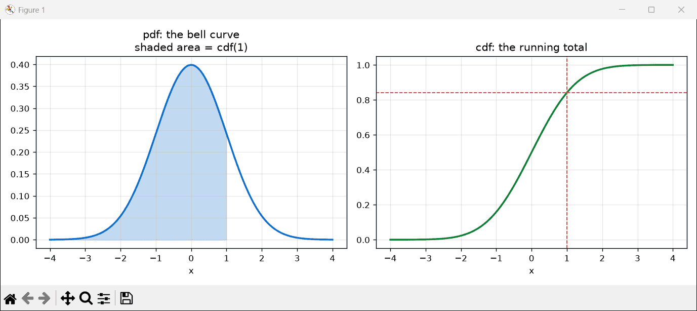
cdf(x) is the running total of the area under the pdf. That is why it rises from 0 to 1 and never falls.
fill_between with a where condition is what shades the region. See Matplotlib plotting for more on styling these.
Using norm.ppf for critical values
ppf is where the numbers in every statistics textbook come from:
from scipy.stats import norm

# ppf is the inverse of cdf: give it a probability, get the value
print("cdf(1.5)        :", round(norm.cdf(1.5), 6))
print("ppf of that     :", round(norm.ppf(norm.cdf(1.5)), 6), "  back where we started")

print()
print("the critical values everyone memorises:")
for confidence in (0.90, 0.95, 0.99):
    z = norm.ppf(1 - (1 - confidence) / 2)
    print(f"  {confidence:.0%} two-sided -> z = {z:.6f}")

print()
print("percentiles of an IQ distribution (mean 100, sd 15):")
for pct in (0.05, 0.25, 0.5, 0.75, 0.95):
    print(f"  {pct:>5.0%} -> {norm.ppf(pct, loc=100, scale=15):.2f}")
Output:
cdf(1.5)        : 0.933193
ppf of that     : 1.5   back where we started

the critical values everyone memorises:
  90% two-sided -> z = 1.644854
  95% two-sided -> z = 1.959964
  99% two-sided -> z = 2.575829

percentiles of an IQ distribution (mean 100, sd 15):
     5% -> 75.33
    25% -> 89.88
    50% -> 100.00
    75% -> 110.12
    95% -> 124.67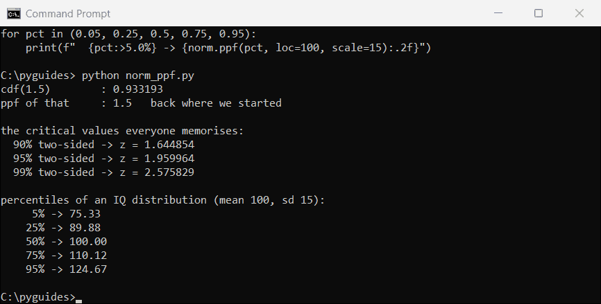
For a two-sided test at 95%, you want the value leaving 2.5% in each tail, which is ppf(0.975).
Getting one-sided and two-sided confused is the classic error here. A one-sided 95% critical value is 1.645, so it’s worth checking which your test needs.
Why 1 – cdf breaks in the tail
This matters for p-values, and it is invisible until it bites:
from scipy.stats import norm

print("in the far tail, 1 - cdf falls apart:")
print(f"{'x':>4} {'1 - cdf(x)':>26} {'sf(x)':>26}")
for x in (2, 5, 10, 20):
    print(f"{x:>4} {1 - norm.cdf(x):>26} {norm.sf(x):>26}")

print()
print("cdf(10) rounds to exactly 1.0 in float64, so the subtraction gives 0.0")
print("sf computes the upper tail directly and keeps its precision")
Output:
in the far tail, 1 - cdf falls apart:
   x                 1 - cdf(x)                      sf(x)
   2        0.02275013194817921       0.022750131948179195
   5      2.866515719235352e-07      2.866515718791933e-07
  10                        0.0       7.61985302416047e-24
  20                        0.0     2.7536241186061556e-89

cdf(10) rounds to exactly 1.0 in float64, so the subtraction gives 0.0
sf computes the upper tail directly and keeps its precision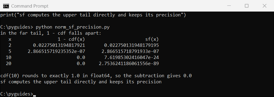
1 - cdf gives exactly 0.0. sf gives 7.6e-24.cdf(10) is so close to 1 that float64 stores it as exactly 1.0. Subtracting that from 1 leaves zero, and every significant digit is gone.
sf computes the upper tail directly, so it keeps its accuracy far past that point. Use it any time you want a small right-tail probability.
The same reasoning applies to logcdf and logsf, which keep working when even sf underflows.
Generating random samples with norm.rvs
rvs draws from the distribution, and random_state makes the draw repeatable:
import numpy as np
from scipy.stats import norm

# random_state makes the draw reproducible
first = norm.rvs(size=5, random_state=42)
second = norm.rvs(size=5, random_state=42)

print("first :", np.round(first, 4))
print("second:", np.round(second, 4))
print("identical:", np.allclose(first, second))

print()
# with a mean and standard deviation, and a shape
sample = norm.rvs(loc=100, scale=15, size=(2, 3), random_state=0)
print("shape (2, 3):")
print(np.round(sample, 2))
Output:
first : [ 0.4967 -0.1383  0.6477  1.523  -0.2342]
second: [ 0.4967 -0.1383  0.6477  1.523  -0.2342]
identical: True

shape (2, 3):
[[126.46 106.   114.68]
 [133.61 128.01  85.34]]
Without random_state you get different numbers every run, which is right for a simulation and wrong for a tutorial or a test.
size accepts a tuple, so you can generate a whole matrix in one call. It behaves like NumPy random generation, which is what it uses underneath.
Confidence intervals with norm.interval
interval gives the central range containing a given share of the distribution:
from scipy.stats import norm

# the central interval containing a given probability
print("standard normal, 95%:", tuple(round(v, 6) for v in norm.interval(0.95)))
print("that 1.96 is where the rule of thumb comes from")

print()
for confidence in (0.90, 0.95, 0.99):
    low, high = norm.interval(confidence, loc=100, scale=15)
    print(f"  {confidence:.0%} of IQ scores fall between {low:.2f} and {high:.2f}")
Output:
standard normal, 95%: (np.float64(-1.959964), np.float64(1.959964))
that 1.96 is where the rule of thumb comes from

  90% of IQ scores fall between 75.33 and 124.67
  95% of IQ scores fall between 70.60 and 129.40
  99% of IQ scores fall between 61.36 and 138.64
norm.interval(0.95) returns -1.96 to 1.96. That is the whole basis of the two-standard-deviation rule of thumb.
With loc and scale it answers the practical question directly, with no manual arithmetic on z-scores.
Fitting a normal distribution with norm.fit
fit estimates the mean and standard deviation from data, and its divisor is worth knowing:
import numpy as np
from scipy.stats import norm

data = norm.rvs(loc=50, scale=8, size=1000, random_state=0)

mean, sd = norm.fit(data)
print(f"norm.fit  -> mean {mean:.6f}, sd {sd:.6f}")

print()
# fit uses maximum likelihood, which divides by n rather than n-1
print(f"np.std(data)          {np.std(data):.6f}   ddof=0")
print(f"np.std(data, ddof=1)  {np.std(data, ddof=1):.6f}   ddof=1, the sample std")
print()
print("fit matches ddof=0:", np.isclose(sd, np.std(data)))
print("so norm.fit gives the population formula, not the sample one")
Output:
norm.fit  -> mean 49.637946, sd 7.896265

np.std(data)          7.896265   ddof=0
np.std(data, ddof=1)  7.900216   ddof=1, the sample std

fit matches ddof=0: True
so norm.fit gives the population formula, not the sample one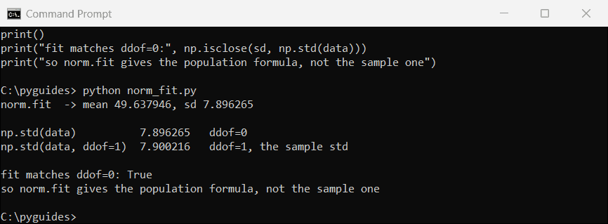
fit matches np.std(data), not np.std(data, ddof=1).fit uses maximum likelihood, which divides by n. The sample standard deviation divides by n – 1.
On 1,000 points the difference is in the fourth decimal place. On 10 points it matters, so use np.std(data, ddof=1) when you want the sample estimate.
Common scipy.stats.norm mistakes
| Symptom | Cause | Fix |
|---|---|---|
| Probabilities look wrong | Variance passed as scale | Pass the standard deviation |
| p-value is exactly 0 | Used 1 - cdf | Use sf |
| Different numbers every run | No random_state | Pass a seed |
| Critical value is 1.645 not 1.96 | One-sided instead of two | Use ppf(0.975) |
fit std differs from yours | MLE divides by n | Compare with ddof=0 |
More SciPy statistics guides:
- The scipy.stats module
- Z-scores with SciPy
- Confidence intervals in SciPy
- Chi-square test
- Independent t-test
- Curve fitting with SciPy
Frequently asked questions
What is scipy.stats.norm used for?
It represents the normal distribution, with methods for the density, the cumulative probability, quantiles and random sampling. The full list is in the scipy.stats.norm reference.
What are loc and scale in scipy.stats.norm?
loc is the mean and scale is the standard deviation. Passing a variance as scale gives a wrong answer with no error.
What is the difference between cdf and ppf?
They are inverses. cdf takes a value and returns a probability; ppf takes a probability and returns the value.
Why does 1 – norm.cdf(x) return 0?
For large x, cdf(x) rounds to exactly 1.0 in floating point, so the subtraction loses everything. Use norm.sf(x) instead.
How do I get reproducible results from norm.rvs?
Pass random_state with a fixed number, such as norm.rvs(size=5, random_state=42).
How do I get a 95% confidence interval?
norm.interval(0.95, loc=mean, scale=sd), which returns the lower and upper bounds directly.
Does norm.fit give the sample standard deviation?
No. It uses maximum likelihood and divides by n, matching np.std(data) rather than np.std(data, ddof=1).

Bijay Kumar is a 13-time Microsoft MVP with more than 18 years in software development, and the founder of Python Guides and TSinfo Technologies. He started out building .NET and SharePoint solutions at HP, TCS and KPIT before moving into Python, machine learning and AI, and he also builds web apps with TypeScript and React. He writes the tutorials here himself, and every example is run before publishing so you see the real output. More about Bijay · Microsoft MVP profile · LinkedIn